


Unit 3: Carbon in the Future & You
3.3: Future Forcings
FOCUS QUESTION:
How are the carbon cycle and humans a part of future climate?
Introduction
In Lesson 3.2, you used the Carbon Connections climate model to compare forcings on Earth's temperature the past 30 years (1979-2010). You tested how four forcings explained most of the temperature record. There are several other possible factors, but the four forcings you used are the best predictors of temperature.
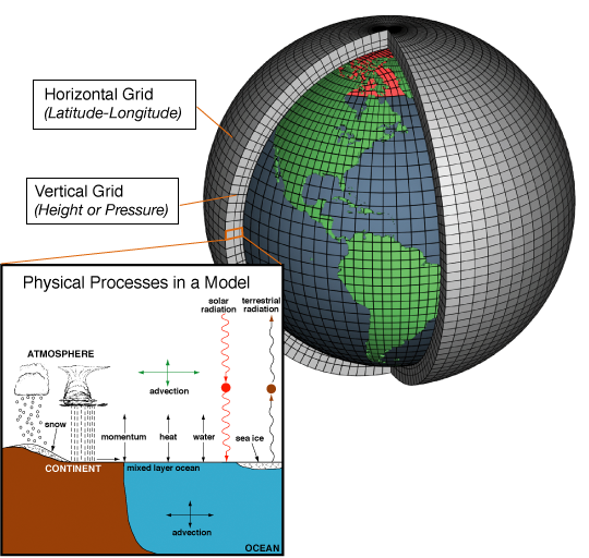
But what does the future hold for Earth's climate? To answer this, scientists use models to make predictions. The models consist of a grid of cells surrounding Earth, similar to the image above. The models determine the transfer of energy and matter among neighboring cells by different physical processes. Using models like this is one vital way to learn what the future might be like.
You will start Lesson 3.3 by summarizing some results from the Carbon Connections climate model. In particular, in this lesson you will see that:
- Variability in the Earth's system over periods of years is different from gradual change in the system over periods of decades.
- Models show how Earth's climate may change in the future with changing CO2 levels in the atmosphere.
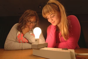
Energy-use monitors help you and your class see how to conserve energy and reduce carbon emissions.
A. What You Saw with the Climate Model
Did you get to show the Carbon Connections climate model to someone in your family? Perhaps they were interested in the climate model and forcing by volcanic aerosols, or perhaps one of the videos of the Sun. Before you consider what might happen in the future, it is good to summarize important things you saw with the climate model. Here are some key points.

First, climate variability tells how much the temperature goes up or down over several months or years. A system can have a lot of variability, yet also have no change in the average. Think of a swing or pendulum. These vary in a back-and-forth manner, but their average position is always the middle. Similarly, the variability of solar cycles is predictable. Solar radiation increases and decreases. In contrast, the El Niño/La Niña cycles show a lot of variability, but when the peaks and valleys occur is less predictable. Volcanic eruptions are even less predictable. These natural forcings lead to variability in temperature.
Second, a key question is whether the Earth's temperature is changing or staying the same. If overall temperature were increasing or decreasing over many years, that would be climate change. Scientists work to tell between climate variability on the scale of years (e.g., El Niño/La Niña cycles), versus climate change over decades. The data you saw in Lesson 3.1 showed a pattern of increasing temperatures, particularly the past 30 years. In Lesson 3.2, the climate model let you test which factor caused that temperature increase. It was the anthropogenic part. In contrast, the "natural" parts of climate variability (that is, solar cycles and El Niño/La Niña cycles) did lead to a net temperature increase over time.
NASA has a short video called "Taking Earth's Temperature" that illustrates some ways that they are working to monitor Earth's climate. Read the questions below and then watch the video.
- Answer the following questions after watching the NASA video:
- What are three major pieces of the climate puzzle that NASA is monitoring?
- Which greenhouse gases are discussed in the video?
- You learned about the reflectivity of volcanic aerosols with the climate model. What is the reflective aerosol discussed in the video?
B. Carbon—Future Forcings
You used one kind of climate model to test climate forcings on Earth's temperature. This model connected increases in CO2 levels in the atmosphere to humans. But you also know from Units 1 and 2 that natural processes also lead to changes in CO2 in the atmosphere. So, how can you test the size of the natural and human processes on the carbon cycle?
At the University of Wisconsin, Professor Galen McKinley has used another kind of model to study the carbon cycle and climate. Her model estimates CO2 levels and temperatures in the future. The trends in CO2 level depend on changes in carbon sources and sinks in the carbon cycle. You studied in Units 1 and 2 processes that change the amount of carbon in the atmosphere. Some processes were related to humans, and others were natural. You will use Professor McKinley's model in the steps below to test the relationship between carbon and climate in the future.
Several key processes affect the total CO2 levels in the atmosphere. In the model, two carbon sources add CO2 to the atmosphere, and two carbon sinks remove CO2 from the atmosphere.
The Global Carbon Budget (University of Wisconsin-Madison)
- Look at the following figure. Answer the questions below about the processes shown that move CO2 into and out of the atmosphere.
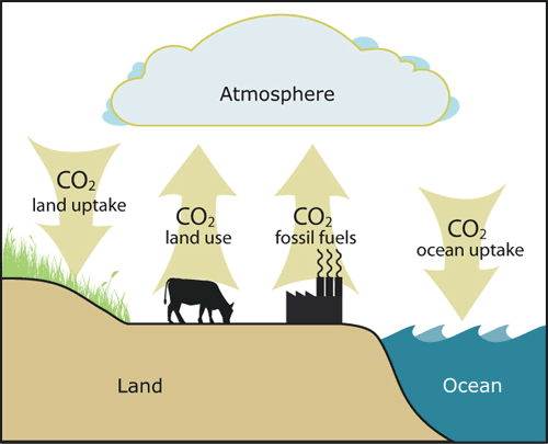
- Carbon sources add CO2 to the atmosphere. Give two examples of carbon sources.
- Carbon sinks remove CO2 from the atmosphere. Give two examples of carbon sinks.
- Recall the Mauna Loa CO2 curve in Unit 2. From that curve, do sources of carbon or sinks of carbon have a greater effect on the amount of carbon in the atmosphere?
- The following information will help you use the carbon budget model.
- Carbon Sinks
- Land Uptake: By keeping forests and soils healthy, land uptake can lead to a net removal of CO2 from the atmosphere. This occurs by photosynthesis. As you saw in Unit 2, respiration does move carbon back to the atmosphere, but the net flow of carbon is to land.
- Ocean Uptake: You saw in Unit 1 that oceans are the largest reservoir of carbon. Uptake of carbon by oceans is probably the most efficient way to remove CO2 from the atmosphere. A possible downside is that CO2 movement to the ocean surface can change the acidity of oceans.
- Carbon Sources
- Land Use: The growing use of land by humans releases carbon from plants, trees, and soils back to the atmosphere. One of the main ways this happens is by converting forests to land for growing crops or grazing. Forest fires also rapidly move carbon from land to the atmosphere.
- Fossil Fuels: Using fossil fuels is important for transportation and generating electrical energy; however, that process leads to a net flow of carbon from where it resides inside Earth to the atmosphere.
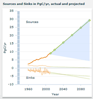
- The figure below shows the first screen of the carbon budget model.
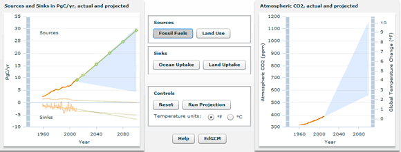
The left graph shows trends in carbon sources and sinks. The right graph shows projections for CO2 in the atmosphere and global temperature. In the left graph, carbon sources have values greater than zero because carbon is added to the atmosphere. Carbon sinks have values that are negative because carbon is subtracted, or removed, from the atmosphere.
Orange parts of the lines show data from 1960 to 2010. The y-axis is petagrams of carbon per year (Pg C/yr). A petagram is a lot of carbon—in fact, one petagram equals 1,000,000,000,000,000 grams of carbon (that is, 1x10¹⁵ grams of carbon). How big is that?! Well, imagine that you had some water. One gram of water is about the size of a sugar cube. But one petagram of water would cover a football field (plus end-zones) with water to a depth of 187 km. That's water 120 miles deep, or about 12 times higher than most of the atmosphere!
In the model, each source or sink has a green curve when you select it. The curves go from 2010 to 2100 and show a set of points. When the curve is selected, you can grab and adjust its trend to simulate different scenarios. You will test some scenarios below. Then, under "Controls," you run your projection to 2100, or reset it to the initial values.
- Follow these steps for a simulation to 2100 using current projections for rate of fuel use.
- Launch the Global Carbon Budget.
- Use the controls to click on Reset. This gives projected trends to 2100 for carbon sources and sinks.
- Click on Run the projection. This will calculate estimated changes in temperature and CO2 levels for those projected trends.
- Record the projected CO2 level for the year 2100.
- Use the steps below for a different scenario. Do a test where the rate of using fossil fuel is reduced by half for 2100. To do that, start with current projections at "Reset," and then do these steps:
- Click on Run Projection for projected trends.
- Next, cut the rate of use in half. Click on Sources on fossil fuels. Grab the highlighted green points on the curve to reduce the slope of the curve by half. For a value in 2100 at 15 Pg C/yr, check that the curve matches the figure below.
- Click on Run Projection. Record the CO2 level for the year 2100.
- Compare CO2 levels between the two runs from Steps 5d and 6c. By cutting the rate of fossil fuel in half, does that stop the increase in CO2 levels in the atmosphere?
- Solutions to climate change rely on not just slowing, but stopping the rate of CO2 growth in the atmosphere. You can test how to do this with the model.
- What shape and trend of the fossil fuel curve gives no increase in CO2 levels?
- How does this pattern of use compare with the data from 1960-2010?
- You can also simulate if the rate of fossil fuel use stayed at today's value (that is, about 9.0 Pg C/yr). Test that scenario with these steps
- Click on Fossil Fuels under Sources. With the highlighted green curve, adjust all points to the value of about 9.0 Pg carbon per year. The green curve will be nearly flat.
- Run the projection. Record the pattern of CO2 levels in the air. If you have a digital notebook, you can also capture the result.
- Explain whether you think that this scenario is realistic. To do that, you can compare constant fossil fuel use to the record from 1960-2010.
- Scientists are concerned that the ability of carbon sinks to keep removing CO2 from the air may decrease. You can models the effect on CO2 levels and temperature if carbon sinks lose their ability to take up carbon at current rates.
- Decide which of the sink curves you will adjust. A flat line means that the sink has stopped taking up more and more carbon each year.
- Adjust the trend of your carbon sink in your model. Record your initial and changed values in your notebook.
- In the steps above, you used the model to test patterns of fossil fuel use and one of the carbon sinks. You can also design your own simulation with more than one source or sink.
- Imagine a country and some decisions or policies that might affect sinks of carbon (land, ocean uptake) or sources of carbon (fossil fuels, land use).
- Record the pattern of sources and sinks that you will simulate.
- What is the effect on CO2 levels in the atmosphere and global temperature?
If you are unable to see the interactive, click here to open it in a new tab.
C. Monitoring Your Use
In Carbon Connections, you have been able to test different kinds of models and interactives. Some have been hands-on, and others have been on a computer. With both of these, you can see a response to an input. At the same time, it is not always as easy to understand how these models for Earth relate to you, your family, and the things you do every day.
The investigations you did in Units 1 and 2 with the energy-use monitor help you see how you can monitor and possibly change your energy use. Electrical energy for humans to use, on average, involves adding carbon to the atmosphere. If you can identify easy ways to use less electrical energy and lower your energy use, you emit less carbon. If many students like you do the same, you all can make a difference.
Home Energy Use Activity
In Units 1 and 2, you used the energy-use monitor. You looked at energy use from different kinds of light bulbs, as well as things in your classroom and school. But what about your home? That's where your family can reduce their energy use. Using less electrical energy means less carbon emissions, and savings to your family on your energy bill.
- Your teacher (or maybe even you!) will bring in a common appliance from home. This could be a hairdryer, radio, cell-phone charger, power drill, room fan, or coffee-maker, for example. Do these steps for that appliance:
- Record the appliance name.
- Describe whether the appliance uses electricity at a steady rate or in cycles. For example, refrigerators cycle on-and-off to keep a steady temperature, while a light uses energy at a steady rate. Describe this pattern.
- Record the rate of energy use in watts. Remember, you can always compare its rate of energy use to that of a 40-watt light bulb.
- Imagine that you got to bring home the energy-use monitor.
- How would you describe its functions to your family?
- What device in your home would you want to check for energy use?
- How would you describe to members of your family the reason why your class was monitoring energy use?
- How could the energy monitor help your family to save money? Depending on the monitor you have in your classroom, it may have a cost option that can be programmed. If not, you can use your electricity bill and an estimate of $0.10 per kilowatt-hour (kWh).
D. Reflect and Connect
- Scientists are concerned that carbon sinks (marine and land ecosystems) may lose their ability to remove carbon from the atmosphere as they are able to do today.
- How would this affect CO2 levels in the atmosphere?
- Can you think of a reason why the ocean might lose its ability to remove carbon from the atmosphere at the same rate?