


Unit 1: Carbon & Climate in the Past
1.4: Global Connections
FOCUS QUESTION:
How can we tell whether climate signals in Earth's past are global or regional in nature?
Introduction
In Lesson 1.3, you studied how forcings cause changes, or responses. One forcing could cause several responses. You also observed how climate scientists, like those at NASA, use climate models to test forcings and responses for Earth's climate. They test the accuracy of such models by changing the level of greenhouse gases in the model atmosphere. For example, they can adjust CO2 levels to match those observed from the Antarctica ice core record. This lets them test how the models match climate variations observed for hundreds of thousands of years. Data from the models and the ice cores match very well.
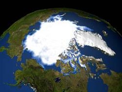
But did those variations of CO2 and climate occur only in Antarctica? If you read Explore More: Carbon Cycle Connections in Lesson 1.2, you saw some maps that showed large changes in Earth's ecosystems between glacial and interglacial periods. In this lesson, you'll analyze other evidence of past climate that you can compare with the Antarctic data. In particular, you will:
- Investigate whether climate signals are global or regional.
- Analyze other indicators of climate cycles on Earth.
- Use models of molecules to simulate physical processes on Earth.
Think about the focus question as you go through this lesson. It will also help you prepare for activities in Lesson 1.5.
A. Evaporation Separation

The water cycle is a key part of understanding Earth's climate. One process of the water cycle is evaporation. Evaporation is where molecules of H2O leave the liquid state to be molecules of H2O vapor in the air. As a vapor, H2O can then move through the atmosphere. As water moves around Earth, it contains a subtle fingerprint of climate. This is because not all water molecules are the same: Some H2O molecules have more mass than other H2O molecules.
Look at the Water Molecules A and B diagrams. Both of these have one oxygen atom and two hydrogen atoms, but they are not the same:
- Molecule A has an oxygen atom with a mass of 16. This comes from 8 protons and 8 neutrons. Each of the two hydrogen atoms has a mass of one. The total mass of Molecule A (H216O) is 16+2, or 18.
- Molecule B has an oxygen atom with a mass of 18. This comes from 8 protons and 10 neutrons. Adding the mass of the two hydrogen atoms gives a total mass for Molecule B (H218O) of 20.
These molecules have different masses because 16O and 18O are two isotopes of oxygen. Two atoms are isotopes if they have the same number of protons, but different numbers of neutrons. This gives them slightly heavier or lighter masses.
Evaporation Table
But how does this relate to processes on Earth? Complete the steps below to model evaporation for H2O molecules with different masses. You may do this as a class, but be sure to record your own answers in your science notebook. Later in the lesson, you will connect this model with patterns of climate on Earth.
- Look at the particles that your teacher has in a box.
- How are the particles similar or different?
- What do the particles represent?
- What do you think is represented by the entire box of particles?
- Imagine that some of the particles were to evaporate and leave the box. With a partner, predict which type of particles would leave the box. Would it be only the heavy or only the light? Be ready to discuss your prediction and reasoning with your class. You will then get to test your prediction.
- Copy headings from the Evaporation table to your science notebook. Count each kind of particle, and enter the totals in the first row. Now, figure out the ratio of heavy-to-light particles (H/L).
| Total | Number of Heavy (H) | Number of Light (L) | Ratio of Heavy to Light (H/L) in Box | |
|---|---|---|---|---|
| Initial | ||||
| In box after shake #1 | ||||
| In box after shake #2 | ||||
| In box after shake #3 |
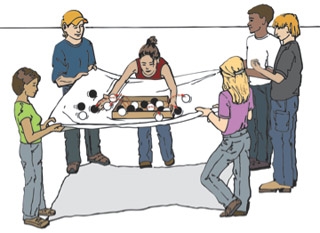
- To model evaporation, a volunteer will shake the box vigorously. Some of the balls will fly out of the box. About four or five volunteers will hold a sheet beneath the box to catch the particles. This is shake #1. Do this for about 10 seconds, or until about one quarter of the particles have bounced out of the box.
- For the particles that left the box, what do you think they represent?
- For the particles still in the box, what do they represent?
- Count the particles left in the box. Record in your table for the groups of total, heavy (H), and light (L).
- Determine the ratio of heavy-to-light particles. You may write this as (H/L) or (H:L). How does this compare with the initial ratio?
- Think about the particles that flew out of the box. Do not put them back in the box.
- If these particles were returned to the box, what would be (H/L) ratio in the box?
- What part of the Earth system could represent the particles returning to the box?
- Now, store them in another container away from the box. What is a region on Earth or process where this could happen?
- What climate conditions would favor the particles being stored somewhere else?
- Repeat step 4 above. This is shake #2. Repeat again for shake #3.
- After recording the results for shake #3, answer these questions.
- How does the initial ratio compare with the ratio after shake #3?
- Return all of the stored particles to the original bin. How does the (H/L) in the box change?
- Overall, what kind of climate conditions do you think would favor particles returning to the box?
- A Features chart can help you connect features of the model with processes or features on Earth. Copy and fill out the table below to help you make those connections. Be sure to add your reasons for the connections in the "because" column.
| Feature of model with foam balls | is like | Feature of Earth system with H2O | because… |
|---|---|---|---|
| Balls without tacks | … | ||
| Balls with tacks | H218O | …when shaking the bin and adding energy, water with the heavy oxygen isotope (18O) is less likely to evaporate and stays in the bin, compared with H216O | |
| … | ice sheets | ||
| Large bin with balls | … | ||
| Sheet gathering flying balls | … | ||
| Energy of shaking | … | ||
| … |
B. Heavy Water
In the last activity, you used a model of the Earth system and the water cycle. The water molecules H216 and H218O behave differently in the water cycle. The lighter H216 evaporates more readily from the ocean than the heavier H218. In the evaporation/shake model, the lighter balls bounced out of the box more easily. The model can also be used to see how changes in the water cycle help geoscientists understand past climate patterns on Earth.
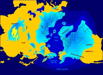
During ice ages (glacial periods, or "glacials"), the amount of ice on Earth was much greater than today. In addition to Antarctica and Greenland, ice sheets covered much of the United States, Canada, and Europe. You saw this in Lesson 1.2. Water that evaporated from the ocean moved over land, and was added to the ice sheets as snowfall. On average, this snow tends to be the low-mass molecule of water, the H216O. When snow falls on the ice sheet, it stays there for a very long time. Thus, the ice sheet stores relatively more H216O than H218O. Conversely, the amount of H218O in the ocean increases compared to the amount of H216O. When water is stored in ice sheets on continents, oceans have more H218O.
In Lesson 1.1, you used an indicator for carbon and CO2 in water. Geoscientists also use an indicator for the amount of H218O in ocean water: δ18O. It's pronounced "delta-18-O." The delta stands for "change," and the 18O represents the 18O in H218O. As with the shaking model, evaporation tends to remove H216O from oceans and store it in ice sheets. As the H218O in oceans increases, the value of δ18O in the ocean also goes up. Ice sheets form in cold climates or during glacial periods. So, glacial periods connect with times of high δ18O in the ocean.
In the past, continental ice sheets were more than 2 kilometers thick in areas of the United States, Canada, and northern Europe and Asia. But these areas are not covered by ice sheets now. Where did the ice sheets go? Think back to where you returned the balls that had shaken out ("evaporated") to the box. You know a process in the water cycle that would return the H2O from ice sheets to the ocean. When ice sheets melt, the H216O returns by rivers to the oceans.
- Add to the table below to summarize the changes in δ18O in the ocean that occur as climate gets warmer or colder.
| Climate | Net Movement of H2O in water cycle | δ18O of oceans (↑ or ↓) |
|---|---|---|
| Cooling to glacial period | Warming to interglacial period | |
| oceans to ice sheets | ice sheets to oceans |
C. Ice Age Proxies
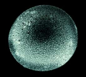
How do geoscientists measure δ18O of ocean water in the past? How do they retrieve evidence of past climate? They get the data from foraminifera, or forams for short. Foraminifera are single-celled organisms that live in the ocean and are a key part of the marine food web. They are widespread in the oceans. Depending on the type, they live in surface waters, or all the way down to the ocean floor. See the example photo of a live foram. When forams die, they fall toward the sea floor and become part of ocean sediments.

A portion of the forams is made up of calcium carbonate (CaCO3). This part of a foram is called a test, and they are very tiny, only about 0.1-1.0 millimeters. Tests are like the shell of a clam, but are on the inside of the organism (that is, the endoskeleton). For the live foram to the left, its test is shown below. After death, this is what forams look like when their organic parts have decayed. These tests can reveal key climate signals.
The oxygen in the CaCO3 that makes up the tests comes from both the H216O and H218O in the oceans. The δ18O of the oxygen in the CaCO3 tells us about Earth's climate during the time when the foram was alive. The δ18O of the tests of forams are a proxy record that tells us about Earth's past climate. Proxy records are data that stand for, or represent, a related feature. Another example of a proxy record is tree rings: The width of tree rings can tell us about yearly rainfall.
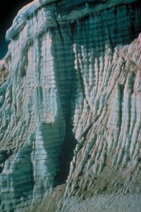
Over thousands of years, foram tests gather with layers of other sediments on the sea floor. This is like the layers of ice you studied. In the ice record, key data is in the ice and trapped air bubbles. From the ocean record, key data is in both the sediments and foram tests in the sediments. When Earth's climate was overall cold, ice sheets grew with water evaporated from the ocean. You saw that the evaporated water had relatively more H216O than the ocean. At the same time, the ocean water was left with relatively more H218O than H216O. This resulted in higher δ18O values for water and foram carbonate.
When Earth's climate warmed, ice sheets began to melt. The water returning to the ocean had relatively higher levels of H216O. This resulted in δ18O values for both the ocean and the foram carbonate to decrease. When lots of foram data are combined, their δ18O values give a proxy record for global ice volume. This pattern is shown in the Global Ice Volume graph. The cycles show changes in ice total ice volume between glacial and interglacial periods. After seeing this graph, you can view an animation again of glacial-interglacial cycles from Lesson 1.2.
- Look at the axes on the Global Ice Volume graph. You will receive a handout of the graph. Write your answers on the graph.
- What is the x-axis? What does it stand for?
- What is the y-axis?
- The value at 440,000 years has a high value of δ18O. Is this a glacial or interglacial period?
- How does the value at 440,000 years compare with the value at 21,000 years?
- The δ18O for current times and 125,000 years ago have low values. Are these glacial or interglacial periods?
- Does Earth show evidence for one big ice age? How many glacial periods, or ice ages, do you count in the last 650,000 years?
- Another proxy for global climate is sea level. This is changes when water is locked in glaciers or is returned to the sea. Complete the two sentences below. They state how δ18O is related to sea level. Enter "high" or "low" for values of δ18O or sea level.
When the Earth's climate was in a glacial period, the sea level was relatively ______________________. This is values of δ18O that are ______________________
When the Earth's climate was in an interglacial period, the sea level was relatively ______________________. This is values of δ18O that are ______________________.
Watch the following video to learn more about forams.
D. Reflect and Connect
You can bring together some ideas from Unit 1 with the following questions. They will help you summarize past changes in climate on Earth.
- Complete the Ice Sheet table to summarize a number of climate effects that you have been discussing. The effects are in the top row. For the first column with ice sheet size, fill in the related climate effects to the right.
Hint: Some relationships are shown in the Climate Records interactive.
| Ice sheet size | CO2 level in atmosphere | Mean global climate | δ18O of oceans | sea level |
|---|---|---|---|---|
| massive | low | |||
| small | ||||
| zero | ||||
| medium |
- Get the Climate Indicators handout from your teacher. Use it to summarize how several factors in the Ice Sheet table connect to the ice volume curve. Add the following phrases to one of the boxes.
| High CO2 | high sea level | warm global temperature | large ice sheets | higher δ18O |
| Low CO2 | low sea level | cool global temperature | small ice sheets | lower δ18O |
- Recall the focus question for this lesson. Do you see climate as being global or regional in nature?
- You have been talking about climate in these lessons. You may not have realized it, but the topics also connect closely with the carbon cycle. Consider the two substances below with carbon. Describe how you think they may be part of the carbon cycle.
- Carbon dioxide (CO2)
- Calcium carbonate (CaCO3)